Advanced Human Activity Classification
This script extends the example from ClassificationAnalysis.m to evaluate other clustering methods. In particular, it addresses:
- Neural Networks
- K Nearest Neighbors
- Naive Bayes
- Linear Discriminant Analysis
- Decision Trees
- Bagged Decision Trees
- Random Forests
- Support Vector Machines
- Ensembles of Learners
- Evaluating and Comparing Classification Solutions
The dataset is courtesy:
Davide Anguita, Alessandro Ghio, Luca Oneto, Xavier Parra and Jorge L.
Reyes-Ortiz. Human Activity Recognition on Smartphones using a
Multiclass Hardware-Friendly Support Vector Machine. International
Workshop of Ambient Assisted Living (IWAAL 2012). Vitoria-Gasteiz,
Spain. Dec 2012
Contents
Load Data
The data is saved in a MAT file. Each row of the variable Xtrain represents one person/instance. The corresponding row of ytrain contains the label of the activity being performed
load Data\HAData

% Set random number generator so results are repeatable
rng(1)
Feature Importance
The complexity of the model and its likelihood to overfit can be reduced by reducing the number of features included. A metric like a paired t test can be used to identify the top features that help separate classes. We can then investigate whether a model trained using only these features can perform comparably with a model trained on the entire dataset
[featIdx, pair] = featureScore(Xtrain, ytrain, 5);

redF = unique(featIdx(:));
features = features(redF);
Xtrain = Xtrain(:,redF);
Xtest = Xtest(:,redF);
Open Pool of Parallel Workers
If Parallel Computing Toolbox is available, the computation will be distributed to 2 workers for speeding up the evaluation.
if isempty(gcp('nocreate'))
    parpool
end
Starting parallel pool (parpool) using the 'local' profile ... connected to 4 workers.
ans =
 Pool with properties:

            Connected: true
           NumWorkers: 4
              Cluster: local
        AttachedFiles: {}
          IdleTimeout: 60 minute(s) (60 minutes remaining)
          SpmdEnabled: true
Neural Networks
Neural Network Toolbox supports supervised learning with feedforward, radial basis, and dynamic networks. It supports both classification and regression algorithms. It also supports unsupervised learning with self-organizing maps and competitive layers.
One can make use of the interactive tools to setup, train and validate a neural network. It is then possible to auto-generate the code for the purpose of automation. In this example, the auto-generated code has been updated to utilize a parallel pool of workers, if available. This is achieved by simply setting the useParallel flag while making a call to train.
[net,~] = train(net,inputs,targets,'useParallel','yes');
If a GPU is available, it may be utilized by setting the useGPU flag.
The trained network is used to make a prediction on the test data and confusion matrix is generated for comparison with other techniques.
net = patternnet(20); % Initialize network

% Setup Division of Data for Training, Validation, Testing
net.divideParam.trainRatio = 70/100;
net.divideParam.valRatio = 15/100;
net.divideParam.testRatio = 15/100;

% Train the Network
net = train(net, Xtrain', dummyvar(ytrain)', 'UseParallel','yes');

scoretest = net(Xtest')';
[~, Y_nn] = max(scoretest,[],2);
C_nn = confusionmat(ytest, Y_nn);
dispConfusion(C_nn, 'Neural Net', labels);
MC_nn = 100 - sum(sum(diag(C_nn)))/sum(sum(C_nn))*100;
fprintf('Overall misclassification rate on test set: %0.2f%%\n',MC_nn)
Performance of model Neural Net:
                                 Predicted WALKING    Predicted WALKING_UPSTAIRS    Predicted WALKING_DOWNSTAIRS    Predicted SITTING    Predicted STANDING    Predicted LAYING
    Actual WALKING               97.78% (485)          1.21% (6)                     1.01% (5)                       0.00% (0)            0.00% (0)             0.00% (0)
    Actual WALKING_UPSTAIRS       7.64% (36)          84.71% (399)                   7.64% (36)                      0.00% (0)            0.00% (0)             0.00% (0)
    Actual WALKING_DOWNSTAIRS     5.71% (24)           7.38% (31)                   86.90% (365)                     0.00% (0)            0.00% (0)             0.00% (0)
    Actual SITTING                0.00% (0)            0.41% (2)                     0.00% (0)                      74.34% (365)         25.25% (124)           0.00% (0)
    Actual STANDING               0.00% (0)            0.19% (1)                     0.00% (0)                      10.34% (55)          89.47% (476)           0.00% (0)
    Actual LAYING                 0.00% (0)            0.00% (0)                     0.00% (0)                       0.00% (0)            0.00% (0)            100.00% (537)
Overall misclassification rate on test set: 10.86%
Classification Using Nearest Neighbors
Categorizing query points based on their distance to points in a training dataset can be a simple yet effective way of classifying new points. Various distance metrics such as euclidean, correlation, hamming, mahalonobis or your own distance metric may be used.
% Train the classifier
knn = fitcknn(Xtrain,ytrain,'Distance','seuclidean','NumNeighbors',10,...
    'PredictorNames',features);

% Make a prediction for the test set
[Y_knn, Yscore_knn] = predict(knn,Xtest);

% Compute the confusion matrix
C_knn = confusionmat(ytest,Y_knn);
dispConfusion(C_knn, 'K Nearest Neighbors', labels);
MC_knn = 100 - sum(sum(diag(C_knn)))/sum(sum(C_knn))*100;
fprintf('Overall misclassification rate on test set: %0.2f%%\n',MC_knn)
Performance of model K Nearest Neighbors:
                                 Predicted WALKING    Predicted WALKING_UPSTAIRS    Predicted WALKING_DOWNSTAIRS    Predicted SITTING    Predicted STANDING    Predicted LAYING
    Actual WALKING               95.77% (475)          2.82% (14)                    1.41% (7)                       0.00% (0)            0.00% (0)             0.00% (0)
    Actual WALKING_UPSTAIRS      12.31% (58)          84.08% (396)                   3.61% (17)                      0.00% (0)            0.00% (0)             0.00% (0)
    Actual WALKING_DOWNSTAIRS     9.76% (41)           8.57% (36)                   81.67% (343)                     0.00% (0)            0.00% (0)             0.00% (0)
    Actual SITTING                0.00% (0)            0.61% (3)                     0.00% (0)                      80.45% (395)         18.94% (93)            0.00% (0)
    Actual STANDING               0.00% (0)            0.19% (1)                     0.00% (0)                      10.34% (55)          89.47% (476)           0.00% (0)
    Actual LAYING                 0.00% (0)            0.00% (0)                     0.00% (0)                       0.00% (0)            0.19% (1)            99.81% (536)
Overall misclassification rate on test set: 11.06%
Naive Bayes Classification
Naive Bayes classification is based on estimating P(X|Y), the probability or probability density of features X given class Y. The Naive Bayes classification object provides support for normal (Gaussian), kernel, multinomial, and multivariate multinomial distributions
% Train the classifier
Nb = fitcnb(Xtrain,ytrain);

% Make a prediction for the test set
Y_nb = predict(Nb,Xtest);

% Compute the confusion matrix
C_nb = confusionmat(ytest,Y_nb);
% Examine the confusion matrix for each class as a percentage of the true class
dispConfusion(C_nb, 'Naive Bayes', labels);
MC_nb = 100 - sum(sum(diag(C_nb)))/sum(sum(C_nb))*100;
fprintf('Overall misclassification rate on test set: %0.2f%%\n',MC_nb)
Performance of model Naive Bayes:
                                 Predicted WALKING    Predicted WALKING_UPSTAIRS    Predicted WALKING_DOWNSTAIRS    Predicted SITTING    Predicted STANDING    Predicted LAYING
    Actual WALKING               92.94% (461)          1.01% (5)                     6.05% (30)                      0.00% (0)            0.00% (0)             0.00% (0)
    Actual WALKING_UPSTAIRS      17.83% (84)          78.56% (370)                   3.61% (17)                      0.00% (0)            0.00% (0)             0.00% (0)
    Actual WALKING_DOWNSTAIRS    16.19% (68)           9.52% (40)                   74.29% (312)                     0.00% (0)            0.00% (0)             0.00% (0)
    Actual SITTING                0.00% (0)            1.22% (6)                     0.00% (0)                      54.38% (267)         44.40% (218)           0.00% (0)
    Actual STANDING               0.00% (0)            0.75% (4)                     0.00% (0)                       4.70% (25)          94.55% (503)           0.00% (0)
    Actual LAYING                 0.00% (0)            0.00% (0)                     0.00% (0)                       0.00% (0)            0.00% (0)            100.00% (537)
Overall misclassification rate on test set: 16.86%
Linear Discriminant Analysis
Discriminant analysis is a classification method. It assumes that different classes generate data based on different Gaussian distributions. Linear discriminant analysis is also known as the Fisher discriminant.
da = fitcdiscr(Xtrain,ytrain,'PredictorNames',features);

% Make a prediction for the test set
[Y_lda, Yscore_lda] = predict(da,Xtest);

% Compute the confusion matrix
C_lda = confusionmat(ytest,Y_lda);
dispConfusion(C_lda, 'LDA', labels);
MC_lda = 100 - sum(sum(diag(C_lda)))/sum(sum(C_lda))*100;
fprintf('Overall misclassification rate on test set: %0.2f%%\n',MC_lda)
Performance of model LDA:
                                 Predicted WALKING    Predicted WALKING_UPSTAIRS    Predicted WALKING_DOWNSTAIRS    Predicted SITTING    Predicted STANDING    Predicted LAYING
    Actual WALKING               95.56% (474)          3.23% (16)                    1.21% (6)                       0.00% (0)            0.00% (0)             0.00% (0)
    Actual WALKING_UPSTAIRS       9.77% (46)          88.96% (419)                   1.27% (6)                       0.00% (0)            0.00% (0)             0.00% (0)
    Actual WALKING_DOWNSTAIRS     5.24% (22)           9.29% (39)                   85.48% (359)                     0.00% (0)            0.00% (0)             0.00% (0)
    Actual SITTING                0.00% (0)            0.00% (0)                     0.00% (0)                      71.89% (353)         28.11% (138)           0.00% (0)
    Actual STANDING               0.19% (1)            0.00% (0)                     0.00% (0)                       7.14% (38)          92.67% (493)           0.00% (0)
    Actual LAYING                 0.00% (0)            0.00% (0)                     0.00% (0)                       0.00% (0)            0.00% (0)            100.00% (537)
Overall misclassification rate on test set: 10.59%
Decision Trees
Classification trees and regression trees are two kinds of decision trees. A decision tree is a flow-chart like structure in which internal node represents test on an attribute, each branch represents outcome of test and each leaf node represents a response (decision taken after computing all attributes). Classification trees give responses that are categorical, such as 'true' or 'false'. Regression trees give numeric responses.
% Train the classifier
t = fitctree(Xtrain,ytrain,'PredictorNames',features);

% Make a prediction for the test set
Y_t = predict(t,Xtest);

% Compute the confusion matrix
C_t = confusionmat(ytest,Y_t);
% Examine the confusion matrix for each class as a percentage of the true class
C_t = dispConfusion(C_t,'Classification Tree',labels);
MC_t = 100 - sum(sum(diag(C_t)))/sum(sum(C_t))*100;
fprintf('Overall misclassification rate on test set: %0.2f%%\n',MC_t)

% view the tree
view(t,'mode','graph')
Performance of model Classification Tree:
                                 Predicted WALKING    Predicted WALKING_UPSTAIRS    Predicted WALKING_DOWNSTAIRS    Predicted SITTING    Predicted STANDING    Predicted LAYING
    Actual WALKING               88.71% (440)          9.88% (49)                    1.41% (7)                       0.00% (0)            0.00% (0)             0.00% (0)
    Actual WALKING_UPSTAIRS      17.20% (81)          74.73% (352)                   8.07% (38)                      0.00% (0)            0.00% (0)             0.00% (0)
    Actual WALKING_DOWNSTAIRS     9.52% (40)          12.62% (53)                   77.86% (327)                     0.00% (0)            0.00% (0)             0.00% (0)
    Actual SITTING                0.20% (1)            0.00% (0)                     0.00% (0)                      71.89% (353)         27.90% (137)           0.00% (0)
    Actual STANDING               0.00% (0)            0.00% (0)                     0.00% (0)                      16.54% (88)          83.46% (444)           0.00% (0)
    Actual LAYING                 0.00% (0)            0.00% (0)                     0.00% (0)                       0.00% (0)            0.00% (0)            100.00% (537)
Overall misclassification rate on test set: 17.22%
Bagged Decision Trees
A single decision tree can be a very easy model to interpret, especially if pruned to a small size. However single trees tend to be poor predictors. Several techniques exist for combining many trees together to improve predictions.
The first is called Bagging, which stands for Bootstrap Aggregation. A series of trees are grown from independent, bootstrapped samples of the input data. To compute prediction for the ensemble of trees, TreeBagger takes an average of predictions from individual trees (for regression) or takes votes from individual trees (for classification). Ensemble techniques such as bagging combine many weak learners to produce a strong learner.
% Train the classifier
ops = statset('UseParallel',true);
tb = TreeBagger(50,Xtrain,ytrain,'method','classification','Options',ops,...
    'NVarToSample','all','PredictorNames',features);

% Make a prediction for the test set
[Y_tb, Yscore_tb] = predict(tb,Xtest);
Y_tb=str2num(cell2mat(Y_tb)); %#ok
% Compute the confusion matrix
C_tb = confusionmat(ytest,Y_tb);
% Examine the confusion matrix for each class as a percentage of the true class
dispConfusion(C_tb, 'Bagged Trees',labels);
MC_tb = 100 - sum(sum(diag(C_tb)))/sum(sum(C_tb))*100;
fprintf('Overall misclassification rate on test set: %0.2f%%\n',MC_tb)
Performance of model Bagged Trees:
                                 Predicted WALKING    Predicted WALKING_UPSTAIRS    Predicted WALKING_DOWNSTAIRS    Predicted SITTING    Predicted STANDING    Predicted LAYING
    Actual WALKING               94.56% (469)          5.04% (25)                    0.40% (2)                       0.00% (0)            0.00% (0)             0.00% (0)
    Actual WALKING_UPSTAIRS      12.95% (61)          83.01% (391)                   4.03% (19)                      0.00% (0)            0.00% (0)             0.00% (0)
    Actual WALKING_DOWNSTAIRS     6.67% (28)          10.48% (44)                   82.86% (348)                     0.00% (0)            0.00% (0)             0.00% (0)
    Actual SITTING                0.00% (0)            0.00% (0)                     0.00% (0)                      74.75% (367)         25.25% (124)           0.00% (0)
    Actual STANDING               0.00% (0)            0.00% (0)                     0.00% (0)                      13.91% (74)          86.09% (458)           0.00% (0)
    Actual LAYING                 0.00% (0)            0.00% (0)                     0.00% (0)                       0.00% (0)            0.00% (0)            100.00% (537)
Overall misclassification rate on test set: 12.79%
Random Forest
Random forests are an extension of bagged decision trees. Random forests only make available a random subset of the predictors for each node in the decision tree to pick from. If a single predictor is much stronger than the others, then it would normally be used very early and often in the tree branching even on indepedently bootstrapped input samples. This correlates the trees and makes them vulnerable to overfitting. By randomizing the predictors available at each node, random forests help to decorrelate the trees. However if the trees are already not correlated then random forests could reduce accuracy by not allowing the tree to use the best possible predictors.
% Train the classifier
rf = TreeBagger(50,Xtrain,ytrain,'method','classification','Options',ops,...
    'PredictorNames',features);

% Make a prediction for the test set
[Y_rf, Yscore_rf] = predict(rf,Xtest);
Y_rf=str2num(cell2mat(Y_rf)); %#ok
% Compute the confusion matrix
C_rf = confusionmat(ytest,Y_rf);
% Examine the confusion matrix for each class as a percentage of the true class
dispConfusion(C_rf, 'Random Forest',labels);
MC_rf = 100 - sum(sum(diag(C_rf)))/sum(sum(C_rf))*100;
fprintf('Overall misclassification rate on test set: %0.2f%%\n',MC_rf)
Performance of model Random Forest:
                                 Predicted WALKING    Predicted WALKING_UPSTAIRS    Predicted WALKING_DOWNSTAIRS    Predicted SITTING    Predicted STANDING    Predicted LAYING
    Actual WALKING               92.74% (460)          6.25% (31)                    1.01% (5)                       0.00% (0)            0.00% (0)             0.00% (0)
    Actual WALKING_UPSTAIRS      13.38% (63)          81.95% (386)                   4.67% (22)                      0.00% (0)            0.00% (0)             0.00% (0)
    Actual WALKING_DOWNSTAIRS     6.67% (28)          11.43% (48)                   81.90% (344)                     0.00% (0)            0.00% (0)             0.00% (0)
    Actual SITTING                0.00% (0)            0.00% (0)                     0.00% (0)                      74.95% (368)         25.05% (123)           0.00% (0)
    Actual STANDING               0.00% (0)            0.00% (0)                     0.00% (0)                      15.60% (83)          84.40% (449)           0.00% (0)
    Actual LAYING                 0.00% (0)            0.00% (0)                     0.00% (0)                       0.00% (0)            0.00% (0)            100.00% (537)
Overall misclassification rate on test set: 13.67%
Support Vector Machines
Support vector machines (SVMs) try to find the hyperplane that best separates the classes. However a single SVM can only work for binary outputs (i.e. yes/no, true/false, etc.) not for multiclass problems. Multiple SVMs can be combined to handle multiclass problems. New in R2014b is the fitcecoc function, which can automatically extend any binary classifier, such as SVMs, to a multiclass problem.
% Train the classifier
svmmdl = templateSVM('KernelFunction','rbf');
mcsvm = fitcecoc(Xtrain,ytrain,'Coding','onevsall','Learners',svmmdl);

% Make a prediction for the test set
[Y_mcsvm, Yscore_mcsvm] = predict(mcsvm,Xtest);
% Compute the confusion matrix
C_mcsvm = confusionmat(ytest,Y_mcsvm);
% Examine the confusion matrix for each class as a percentage of the true class
dispConfusion(C_mcsvm, 'Support Vector Machine',labels);
MC_mcsvm = 100 - sum(sum(diag(C_mcsvm)))/sum(sum(C_mcsvm))*100;
fprintf('Overall misclassification rate on test set: %0.2f%%\n',MC_mcsvm)
Performance of model Support Vector Machine:
                                 Predicted WALKING    Predicted WALKING_UPSTAIRS    Predicted WALKING_DOWNSTAIRS    Predicted SITTING    Predicted STANDING    Predicted LAYING
    Actual WALKING               95.16% (472)          4.64% (23)                    0.20% (1)                       0.00% (0)            0.00% (0)             0.00% (0)
    Actual WALKING_UPSTAIRS      12.74% (60)          85.56% (403)                   1.70% (8)                       0.00% (0)            0.00% (0)             0.00% (0)
    Actual WALKING_DOWNSTAIRS     5.71% (24)           8.10% (34)                   86.19% (362)                     0.00% (0)            0.00% (0)             0.00% (0)
    Actual SITTING                0.00% (0)            0.00% (0)                     0.00% (0)                      75.97% (373)         22.81% (112)           1.22% (6)
    Actual STANDING               0.00% (0)            0.00% (0)                     0.00% (0)                       9.21% (49)          90.60% (482)           0.19% (1)
    Actual LAYING                 0.00% (0)            0.00% (0)                     0.00% (0)                       0.00% (0)            0.00% (0)            100.00% (537)
Overall misclassification rate on test set: 10.79%
Combine Classifiers
There are different heuristic methods that can be used to combine classifiers. Formal ensemble learning methods train a group of classifiers in a systematic way to improve their combined performance. Bagging is one method as is Boosting. The fitensemble method provides a number of these techniques. A simpler method that is often used in practice is to combine the outputs of independently trained classifiers through either a voting scheme or by combining predictor scores.
% Combine four best techniques through simple voting scheme
comb = [Y_nn,Y_knn,Y_lda,Y_mcsvm];
Y_mode = mode(comb,2);
% Compute the confusion matrix
C_mode = confusionmat(ytest,Y_mode);
% Examine the confusion matrix for each class as a percentage of the true class
dispConfusion(C_mode, 'Voting Scheme',labels);
MC_mode = 100 - sum(sum(diag(C_mode)))/sum(sum(C_mode))*100;
fprintf('Overall misclassification rate on test set: %0.2f%%\n',MC_mode)
Performance of model Voting Scheme:
                                 Predicted WALKING    Predicted WALKING_UPSTAIRS    Predicted WALKING_DOWNSTAIRS    Predicted SITTING    Predicted STANDING    Predicted LAYING
    Actual WALKING               98.19% (487)          1.41% (7)                     0.40% (2)                       0.00% (0)            0.00% (0)             0.00% (0)
    Actual WALKING_UPSTAIRS      10.62% (50)          87.26% (411)                   2.12% (10)                      0.00% (0)            0.00% (0)             0.00% (0)
    Actual WALKING_DOWNSTAIRS     6.19% (26)           8.33% (35)                   85.48% (359)                     0.00% (0)            0.00% (0)             0.00% (0)
    Actual SITTING                0.00% (0)            0.41% (2)                     0.00% (0)                      76.17% (374)         23.42% (115)           0.00% (0)
    Actual STANDING               0.00% (0)            0.19% (1)                     0.00% (0)                      10.15% (54)          89.66% (477)           0.00% (0)
    Actual LAYING                 0.00% (0)            0.00% (0)                     0.00% (0)                       0.00% (0)            0.00% (0)            100.00% (537)
Overall misclassification rate on test set: 10.25%
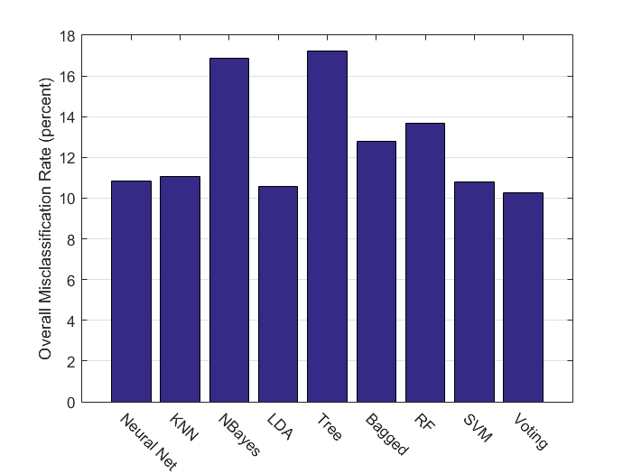
Compare Models with Misclassification Rates
There are many different ways to compare the accuracy and effectiveness of different classifiers. Here we look simply at the overall misclassification rate, and see that voting scheme perfomed best followed by the Support Vector Machines.
methods = {'Neural Net','KNN','NBayes','LDA','Tree','Bagged','RF','SVM','Voting'};
MC_comb = [MC_nn,MC_knn,MC_nb,MC_lda,MC_t,MC_tb,MC_rf,MC_mcsvm,MC_mode];
bar(MC_comb);set(gca,'YGrid', 'on','XTickLabel',methods,'XTickLabelRotation',-45);
ylabel('Overall Misclassification Rate (percent)')