Advanced Human Activity Clustering
This script extends the example from ClusterAnalysis.m to evaluate other clustering methods. In particular, it addresses: * Hierarchical Clustering, Dendrograms & Cophenetic Correlation * Fuzzy C-means Clustering (Fuzzy Logic Toolbox) * Self-Organizing Maps (Neural Network Toolbox) * Evaluating & Comparing Clustering Solutions
The dataset is courtesy:
Davide Anguita, Alessandro Ghio, Luca Oneto, Xavier Parra and Jorge L.
Reyes-Ortiz. Human Activity Recognition on Smartphones using a
Multiclass Hardware-Friendly Support Vector Machine. International
Workshop of Ambient Assisted Living (IWAAL 2012). Vitoria-Gasteiz,
Spain. Dec 2012
Contents
Load Data
Load Human-Activity dataset for clustering.
load Data\HAData Xtrain features

% Perform PCA decomposition
[coeff,score,latent] = pca(Xtrain);
Initial Clustering Solution Baseline
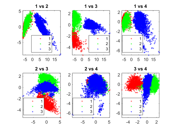
Compute initial K-means clustering solution for comparison
rng(1)
kidx = kmeans(Xtrain, 3, 'distance', 'correlation', 'replicates', 5);
Hierarchical Clustering, Cophenetic Corr. Coeff. and Dendrogram
Hierarchical Clustering groups data over a variety of scales by creating a cluster tree or dendrogram. The tree is not a single set of clusters, but rather a multilevel hierarchy, where clusters at one level are joined as clusters at the next level. A variety of distance measures such as Euclidean, Mahalanobis, Jaccard etc. are available.
Cophenetic correlation coefficient is typically used to evaluate which type of hierarchical clustering is more suitable for a particular type of data. It is a measure of how faithfully the tree represents the similarities/dissimilarities among observations.
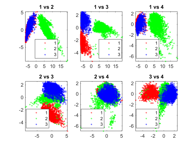
Dendrogram is a graphical representation of the cluster tree created by hierarchical clustering.
Z = linkage(score(:,1:8), 'ward');
hidx = cluster(Z, 'maxclust', 3);
pairscatter(score(:,1:4), [], hidx)
Fuzzy C-Means
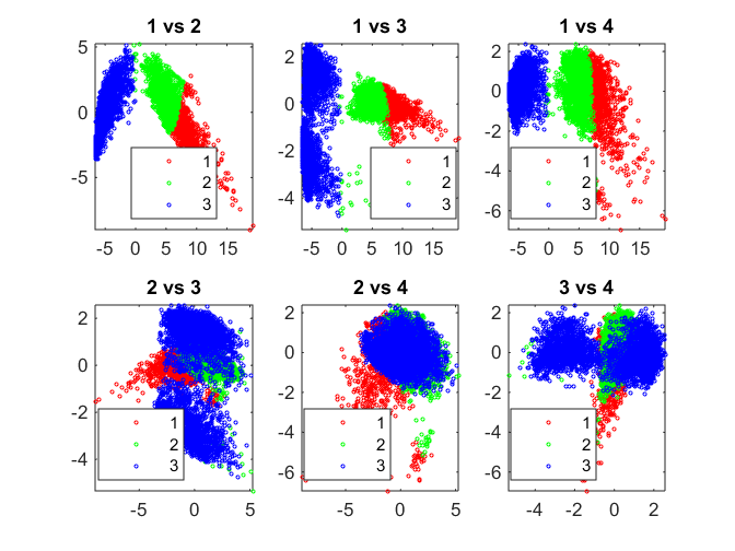
Fuzzy C-means (FCM) is a data clustering technique wherein each data point belongs to a cluster to some degree that is specified by a membership grade. The function fcm returns a list of cluster centers and several membership grades for each data point.
fcm iteratively minimizes the sum of distances of each data point to its cluster center weighted by that data point's membership grade.
[center,U] = fcm(score(:,1:8), 3);

% Generate hard clustering for evaluation
[~, fidx] = max(U);
fidx = fidx';
pairscatter(score(:,1:4), [], fidx)
Iteration count = 1, obj. fcn = 137819.579437
Iteration count = 2, obj. fcn = 107281.114182
Iteration count = 3, obj. fcn = 106944.221021
Iteration count = 4, obj. fcn = 103944.473308
Iteration count = 5, obj. fcn = 85623.085511
Iteration count = 6, obj. fcn = 60847.812140
Iteration count = 7, obj. fcn = 57132.202217
Iteration count = 8, obj. fcn = 56342.025480
Iteration count = 9, obj. fcn = 55881.538183
Iteration count = 10, obj. fcn = 55379.297388
Iteration count = 11, obj. fcn = 54930.558578
Iteration count = 12, obj. fcn = 54645.521084
Iteration count = 13, obj. fcn = 54504.706074
Iteration count = 14, obj. fcn = 54440.348551
Iteration count = 15, obj. fcn = 54406.185557
Iteration count = 16, obj. fcn = 54380.022611
Iteration count = 17, obj. fcn = 54351.219593
Iteration count = 18, obj. fcn = 54313.047763
Iteration count = 19, obj. fcn = 54259.596197
Iteration count = 20, obj. fcn = 54185.188121
Iteration count = 21, obj. fcn = 54085.785091
Iteration count = 22, obj. fcn = 53962.397562
Iteration count = 23, obj. fcn = 53824.908242
Iteration count = 24, obj. fcn = 53691.594492
Iteration count = 25, obj. fcn = 53580.954715
Iteration count = 26, obj. fcn = 53501.834614
Iteration count = 27, obj. fcn = 53451.711405
Iteration count = 28, obj. fcn = 53422.533283
Iteration count = 29, obj. fcn = 53406.404596
Iteration count = 30, obj. fcn = 53397.740578
Iteration count = 31, obj. fcn = 53393.154589
Iteration count = 32, obj. fcn = 53390.744938
Iteration count = 33, obj. fcn = 53389.483464
Iteration count = 34, obj. fcn = 53388.824343
Iteration count = 35, obj. fcn = 53388.480329
Iteration count = 36, obj. fcn = 53388.300904
Iteration count = 37, obj. fcn = 53388.207367
Iteration count = 38, obj. fcn = 53388.158622
Iteration count = 39, obj. fcn = 53388.133225
Iteration count = 40, obj. fcn = 53388.119996
Iteration count = 41, obj. fcn = 53388.113106
Iteration count = 42, obj. fcn = 53388.109518
Iteration count = 43, obj. fcn = 53388.107650
Iteration count = 44, obj. fcn = 53388.106677
Iteration count = 45, obj. fcn = 53388.106171
Iteration count = 46, obj. fcn = 53388.105907
Iteration count = 47, obj. fcn = 53388.105770
Iteration count = 48, obj. fcn = 53388.105698
Iteration count = 49, obj. fcn = 53388.105661
Iteration count = 50, obj. fcn = 53388.105642
Iteration count = 51, obj. fcn = 53388.105631
Iteration count = 52, obj. fcn = 53388.105626
Neural Networks - Self Organizing Maps (SOMs)
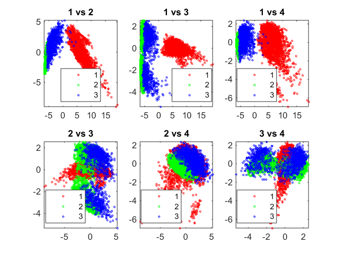
Neural Network Toolbox supports unsupervised learning with self-organizing maps (SOMs) and competitive layers.
SOMs learn to classify input vectors according to how they are grouped in the input space. SOMs learn both the distribution and topology of the input vectors they are trained on. One can make use of the interactive tools to setup, train and test a neural network. It is then possible to auto-generate the code for the purpose of automation. The code in this section has been auto-generated.
% Create a Self-Organizing Map
dimension1 = 3;
dimension2 = 1;
net = selforgmap([dimension1 dimension2]);

% Train the Network
net.trainParam.showWindow = 1;
[net,tr] = train(net, Xtrain');

% Test the Network
nidx = net(Xtrain');
nidx = vec2ind(nidx)';

% Visualize results
pairscatter(score(:,1:4),[],nidx);
Gaussian Mixture Models (GMM)
Gaussian mixture models are formed by combining multivariate normal density components. gmdistribution.fit uses expectation maximization (EM) algorithm, which assigns posterior probabilities to each component density with respect to each observation. The posterior probabilities for each point indicate that each data point has some probability of belonging to each cluster.
gmobj = fitgmdist(score(:,1:8), 3, 'Replicates', 5);
gidx = cluster(gmobj, score(:,1:8));

pairscatter(score(:,1:4), [], gidx);
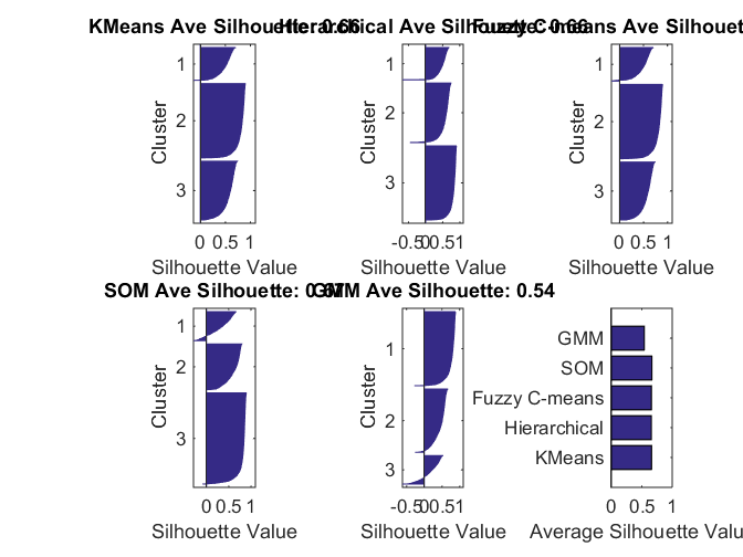
Cluster Evaluation
Compare clustering solutions using average silhouette value. This is one objective criterion. It may not guarantee the best clustering solution, which can be a subjective determination.
sols = [kidx hidx fidx nidx gidx];
methods = {'KMeans','Hierarchical','Fuzzy C-means','SOM','GMM'};
silAve = zeros(1, size(sols,2));
for i = 1:size(sols,2)
    subplot(2,3,i);
    %[silh,~] = silhouette(Xtrain, sols(:,i), 'correlation');
    [silh,~] = silhouette(score(:,1:8), sols(:,i));
    silAve(i) = mean(silh);
    title(sprintf('%s Ave Silhouette: %0.2f', methods{i}, silAve(i)));
end
subplot(2,3,6);
barh(silAve); xlabel('Average Silhouette Value');
set(gca,'YTick', 1:length(silAve), 'YTickLabel', methods);
Determining Number of Clusters
The evalclusters function can be used to evaluate a clustering algorithm like kmeans for different number of clusters and calculate a metric that can be used to determine the optimal number of clusters.
Notice that here, for both kmeans and hierarchical clustering, the optimal number of clusters is 2.
ev1 = evalclusters(score(:,1:8),'kmeans','CalinskiHarabasz','KList',2:6)
ev2 = evalclusters(score(:,1:6),'kmeans','DaviesBouldin','KList',2:6)

ev1 = evalclusters(score(:,1:8),'linkage','CalinskiHarabasz','KList',2:6)
ev2 = evalclusters(score(:,1:6),'linkage','DaviesBouldin','KList',2:6)
ev1 =
  CalinskiHarabaszEvaluation with properties:

    NumObservations: 7352
         InspectedK: [2 3 4 5 6]
    CriterionValues: [1.9534e+04 1.2766e+04 1.1405e+04 9.9601e+03 8.9938e+03]
           OptimalK: 2
ev2 =
  DaviesBouldinEvaluation with properties:

    NumObservations: 7352
         InspectedK: [2 3 4 5 6]
    CriterionValues: [0.5312 0.9129 1.1035 1.0865 1.1257]
           OptimalK: 2
ev1 =
  CalinskiHarabaszEvaluation with properties:

    NumObservations: 7352
         InspectedK: [2 3 4 5 6]
    CriterionValues: [1.9403e+04 1.2426e+04 1.0694e+04 9.0625e+03 8.0660e+03]
           OptimalK: 2
ev2 =
  DaviesBouldinEvaluation with properties:

    NumObservations: 7352
         InspectedK: [2 3 4 5 6]
    CriterionValues: [0.5323 0.9626 1.1654 1.0866 1.1405]
           OptimalK: 2