Contents

Clustering Human Activity Sensor Data

Human activity sensor data contains observations derived from sensor measurements taken from smartphones worn by people while doing different activities (walking, lying, sitting). The series of measurements were run through a feature extractor to compute 561 attributes per observation. The goal of this analysis is to identify clusters of similar activities and what they may represent.

The dataset is courtesy:
Davide Anguita, Alessandro Ghio, Luca Oneto, Xavier Parra and Jorge L.
Reyes-Ortiz. Human Activity Recognition on Smartphones using a
Multiclass Hardware-Friendly Support Vector Machine. International
Workshop of Ambient Assisted Living (IWAAL 2012). Vitoria-Gasteiz,
Spain. Dec 2012

% Copyright 2014 MathWorks, Inc.

Load Data

The data is saved in a MAT file. Each row of the variable Xtrain represents one person/instance. Clusters can be found by grouping similar rows of Xtrain. The list of 561 features is also imported.

%load Data\HAData Xtrain features

Xtrain = importXdata('Data/X_train.txt');
features = importfeatures('Data/features.txt');

Visualize dataset

This dataset has 561 columns or variables making it a high-dimensional dataset that is inherently hard to visualize. We must therefore choose certain columns of data or reduce the number of dimensions

Dimensionality Reduction - PCA

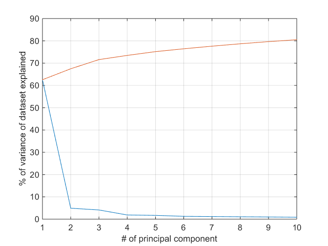
Principal component analysis (PCA) is one of the most popular methods of reducing the dimensionality of the data by computing orthogonal dimensions of maximum variance of the dataset. In this case, note that a few principal components capture a good portion of the variance in the dataset but that variance captured doesn't grow very fast with an increase in the number of principal components.

[coeff,score,latent] = pca(Xtrain);

clf
plot([latent(1:10)/sum(latent) cumsum(latent(1:10))/sum(latent)]*100);
xlabel('# of principal component');
ylabel('% of variance of dataset explained');
grid on

Visualize Clustering Using Reduced Data

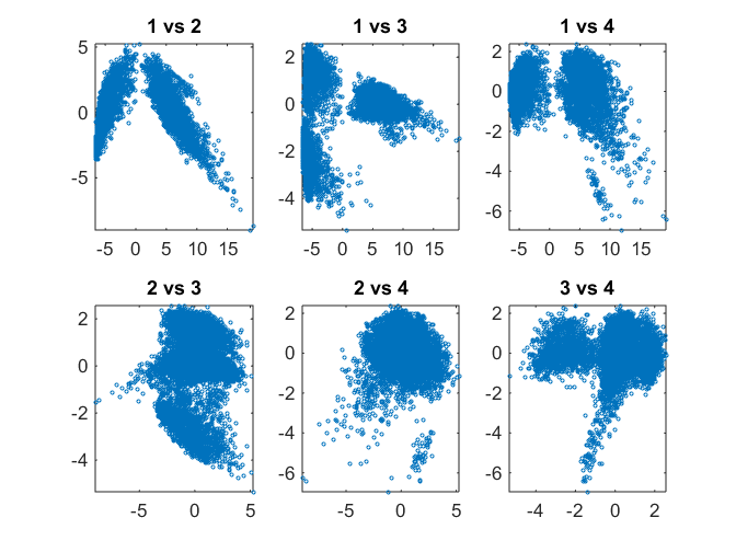
We can perform a pairwise scatter plots of the scores (loadings) of each observation for a few principal components. In addition to plotting the points, we calculate and plot the density at each point using a heatmap so that the structure of the dataset becomes apparent. Alex Sanchez's scatplot (http://www.mathworks.com/matlabcentral/fileexchange/8577-scatplot) is used for this purpose. One can start to identify clusters visually from this plot.

pairscatter(score(:,1:4),[],[],'showdensity', false);

K-Means Clustering

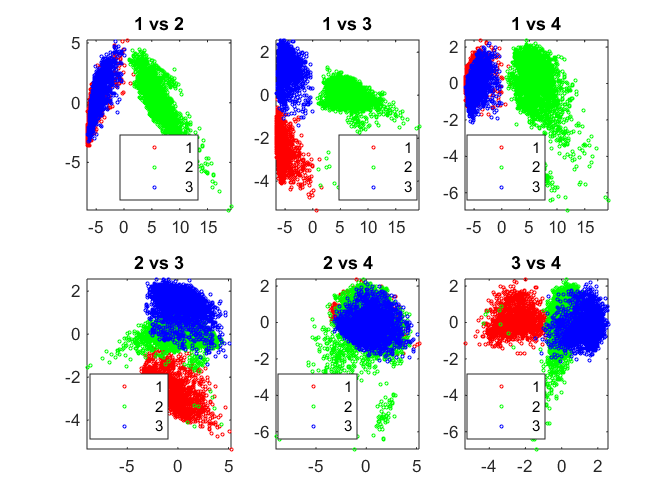
Perform K-means clustering to identify 3 clusters in the data set. The correlation distance metric is used and the clustering is performed 5 times with different initial guesses (to prevent local minima solutions).

We can visualize cluster identity using a colored pair-scatter plot on the PCA scores.

rng default
nClust = 3;
kidx = kmeans(Xtrain, nClust, 'distance', 'correlation', 'replicates', 5);

pairscatter(score(:,1:4), [], kidx);

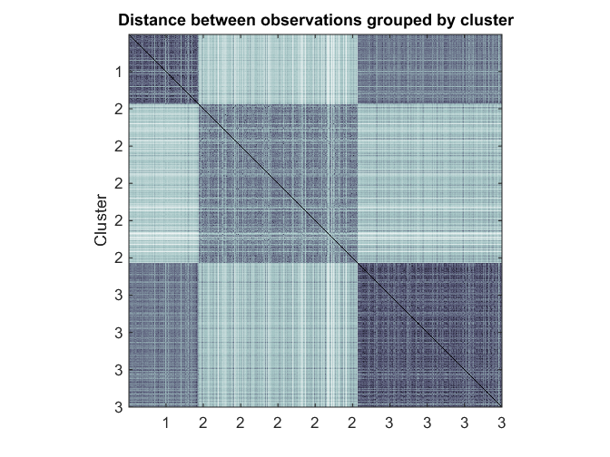
Cluster Evaluation - Visualization of Similarity

One method of evaluating the clustering is to visualize the matrix of distances sorted by cluster membership. This can help easily visualize within-cluster and between-cluster distances between groups.

Here, because visualizing 7352^2 points is overkill, we will sample 1000 points from the dataset uniformly without replacement.

% Sample 1000 points uniformly
Nsample = 1000;
[Xsample, ind] = datasample(Xtrain, Nsample, 'Replace', false);
ksample = kidx(ind);

% Compute pairwise distances
dists = pdist(Xsample, 'correlation');
Z = squareform(dists);

% Visualize cluster similarity by using a heatmap
[~,idx] = sort(ksample);
figure
heatmap(Z(idx,idx),ksample(idx),ksample(idx),[],'colormap',@bone,'uselogcolormap',true);
ylabel('Cluster')
title('Distance between observations grouped by cluster')
axis square

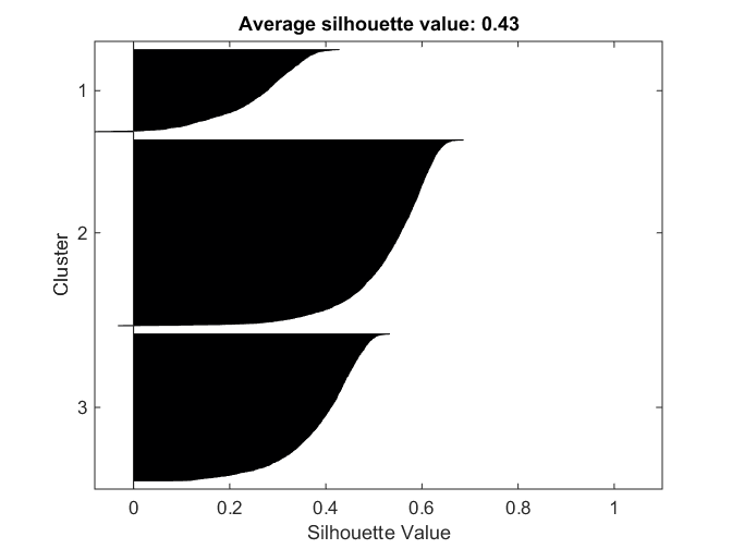
Cluster Evaluation - Silhouette Value

Another metric for evaluating clusters is the silhouette value. This is a measure of how close each point in one cluster is to points in the neighboring clusters. This measure ranges from +1, indicating points that are very distant from neighboring clusters, through 0, indicating points that are not distinctly in one cluster or another, to -1, indicating points that are probably assigned to the wrong cluster.

The silhouette plot plots the sorted silhouette values for each point in a cluster, grouped by cluster. We also compute the average silhouette values in each case.

[sil,~] = silhouette(Xtrain, kidx, 'correlation');
title(sprintf('Average silhouette value: %0.2f', mean(sil)));

Find Discriminative Features

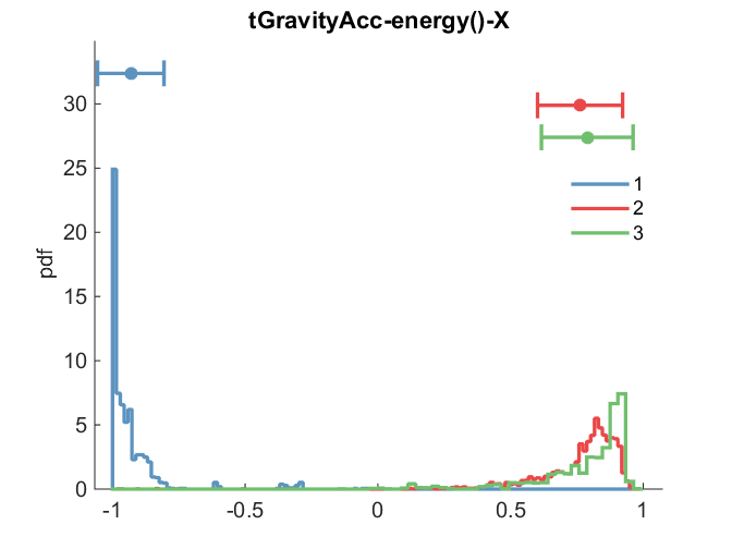
It can be helpful to find a small set of features that can highly discriminate between clusters. This can reduce the dimensionality of the problem and help in interpreting the clustering results as we will see later. To do that, we use a function that computes a paired t test for each feature for each cluster pair and uses the test statistic to rank the features.

[featIdx, pair] = featureScore(Xtrain, kidx, 10);

disp('Top features for separation of clusters:');
for i = 1:size(pair,1)
    fprintf('%d and %d: ', pair(i,1), pair(i,2));
    fprintf('%s, ', features{featIdx(i,:)});
    fprintf('\n');
end

Top features for separation of clusters:
1 and 2: tGravityAcc-energy()-X, tBodyAccJerkMag-entropy(), fBodyAccJerk-entropy()-X, tBodyAccJerk-entropy()-X, tGravityAcc-mean()-X, tGravityAcc-max()-X, fBodyAccJerk-entropy()-Y, tBodyAccJerk-entropy()-Y, angle(X,gravityMean), tGravityAcc-min()-X, 
1 and 3: tGravityAcc-energy()-X, tGravityAcc-mean()-X, tGravityAcc-min()-X, angle(X,gravityMean), tGravityAcc-max()-X, tGravityAcc-energy()-Y, tGravityAcc-max()-Y, tGravityAcc-mean()-Y, angle(Y,gravityMean), tGravityAcc-min()-Y, 
2 and 3: fBodyAccJerk-entropy()-X, tBodyAccJerkMag-entropy(), fBodyAcc-entropy()-X, fBodyAccJerk-entropy()-Y, tBodyAccJerk-entropy()-X, tBodyAccJerk-entropy()-Y, tBodyAccJerk-entropy()-Z, fBodyBodyAccJerkMag-entropy(), fBodyAcc-entropy()-Y, fBodyAccMag-entropy(), 

We can visually confirm the separation of clusters by feature using a grouped histogram plot

f = 57;
clf
nhist(grpSplit(Xtrain(:,f), kidx), 'legend', cellstr(int2str((1:nClust)')));
title(features{f});

Attribute Meaning to Clusters

What do the clusters represent? One way of attributing meaning is to use the discriminative features to characterize each cluster. For example, if one cluster has a really high or low average for a feature a physical interpretation for that cluster can be made. Here, we calculate the mean value of each highly discriminative feature grouped by cluster and present it in a tabular and heatmap view for interpretation.

allF = unique(featIdx(:));
g = grpstats(Xtrain(:,allF),kidx)';
featMeans = table(features(allF), g, 'VariableNames', {'Feature', 'ClusterMeans'});
display(featMeans);

heatmap(g,1:nClust,features(allF),'%0.1f','gridlines','-','showAllTicks',true);
colormap copper
colorbar
xlabel Cluster

featMeans = 
                Feature                             ClusterMeans             
    _______________________________    ______________________________________
    'tGravityAcc-mean()-X'               -0.34474        0.9082       0.91917
    'tGravityAcc-mean()-Y'                0.62828      -0.21617     -0.046546
    'tGravityAcc-max()-X'                -0.39142       0.84992       0.84968
    'tGravityAcc-max()-Y'                 0.59607      -0.22079     -0.063055
    'tGravityAcc-min()-X'                -0.31161        0.9139       0.93407
    'tGravityAcc-min()-Y'                 0.63374      -0.20359      -0.03095
    'tGravityAcc-energy()-X'             -0.93119       0.76233       0.78927
    'tGravityAcc-energy()-Y'           -0.0048112      -0.89987      -0.92147
    'tBodyAccJerk-entropy()-X'           -0.64412       0.60251      -0.68328
    'tBodyAccJerk-entropy()-Y'           -0.67273       0.58051      -0.64027
    'tBodyAccJerk-entropy()-Z'           -0.67147       0.52203      -0.66279
    'tBodyAccJerkMag-entropy()'          -0.71784       0.70824      -0.70437
    'fBodyAcc-entropy()-X'                -0.7921       0.56775      -0.87102
    'fBodyAcc-entropy()-Y'                -0.8077       0.51569      -0.74694
    'fBodyAccJerk-entropy()-X'           -0.94168       0.53686      -0.94019
    'fBodyAccJerk-entropy()-Y'           -0.92985       0.52114      -0.91437
    'fBodyAccMag-entropy()'              -0.79036       0.52176      -0.77751
    'fBodyBodyAccJerkMag-entropy()'      -0.93421       0.36986      -0.92778
    'angle(X,gravityMean)'                0.49709      -0.72056      -0.74871
    'angle(Y,gravityMean)'               -0.43508       0.23258       0.11437

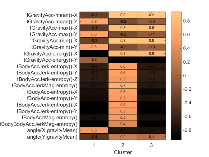
Notice that cluster 2 has high values for body acceleration entropy and body acc jerk entropy in all dimensions whereas clusters 1 and 3 have low values. This suggests that cluster 2 represents instances where the person is engaged in a lot of motion and clusters 1 and 3 contain instances of being still.

The difference between clusters 1 and 3 are apparent from the gravity acceleration features. Cluster 3 (and 2) has high average gravity acceleration in the X direction (low in Y) while cluster 1 has higher values in the Y direction. This would suggest that cluster 3 represents being upright but still whereas cluster 1 represents being horizontal (laying) and still. The average values for the angle(X,gravityMean) feature further suggest this hypothesis.

Cluster interpretation:

Published with MATLAB® R2014b